Predicting Alpha Portfolio

Research created using data from Jan 04, 2011 to October 17, 2025

The TL;DR Version

The Predicting Alpha portfolio combines two simple systems used in professional investing:

1. A diversified multi-asset ETF portfolio

Inspired by Ray Dalio’s “All Weather” approach, enhanced with a momentum overlay to help avoid major downturns.

2. A volatility strategy

Shorting VXX in calm markets to capture the volatility risk premium, and flipping long volatility during stressed markets.

Together these two systems create a portfolio that historically delivered:

• 18.40% annual returns
• 15% volatility, lower than equities
• 20% maximum drawdown
• Strong risk-adjusted returns (1.22 Sharpe)

The system takes just minutes per week to run.

Everything in this portfolio is built on transparent logic and well-documented research.

What is in the rest of this document?

The rest of this document walks through every decision behind the system — the portfolio construction, the signals that drive trades, how positions are sized, and the assumptions used in testing — so you can understand exactly how the machine works.

If you prefer to just run the system, the platform handles the calculations for you. But if you want to know what’s under the hood, every piece of data, logic, test, and assumption is covered below.

Introduction

The Predicting Alpha Portfolio is designed to provide retail traders with a way to trade and invest their money that they can feel confident using not only today, but for the years to come.

Note: In this document we explain the research, logic, and calculations that go into creating this portfolio to help you understand what is going on under the hood. All of these calculations are handled for you in the paper, so do not get intimidated by it as you read further.

To achieve the financial goals that most of us started this journey with, we need a couple of key things

1. A way to allocate our capital where we can feel confident that it will grow faster and with less risk than just the market
2. Enough confidence to continue adding money to the portfolio to accelerate the growth
3. Enough time for the compounding effect to play out

If we knew that the trading/investing decisions we were making accomplished these three things, we would be in an incredible financial position.

The challenge with this is that our options for how to accomplish these points are limited and ineffective. It’s rare to see a retail trader stick with a strategy for 6 months, let alone 6 years. Oftentimes this is because the strategy they followed didn’t actually have the expected returns they thought it did, but other times it’s honestly because there weren’t clear and realistic expectations to begin with.

Portfolio Objective

The purpose of this portfolio is to give you a realistic way to grow your capital at rates that exceed market average returns while simultaneously taking less risk.

We define realistic as:

1. Is well documented and used in the professional space too.
2. Is likely to continue working for many years.
3. Logically it makes sense why the strategy is profitable (no magic).
4. The logic is verified through data analysis and a clear edge is observable.
5. Does not require you to be a professional (deep understanding of math, trade execution, or having very expensive equipment).
6. Has enough capacity that a group of traders could reasonably use it with larger sums of capital (since that is the goal).

We defined success for the Predicting Alpha Project as the creation of a portfolio that caters successfully and precisely to the needs of self directed investors. It must not only demonstrate a superior return profile (CAGR, risk, volatility) to other available options, it must also be realistic for you to trade it successfully (time commitments, complexity, getting the same fill prices as in testing, etc).

By the end of this document you should have the confidence needed to move forward today with allocating meaningful capital to this incredible portfolio, which can serve as a bedrock for your investments and deliver the results you originally expected when getting into trading.

Portfolio Overview

This portfolio consists of two complementary strategies. Our ETF Strategy, and our VIX strategy.

1. ETF Strategy: An “All Weather” ETF basket with a signal to avoid major downturns
2. A short VXX strategy with a signal to flip long when market volatility picks up.

ETF + VIX Strategies Portfolio Performance Chart

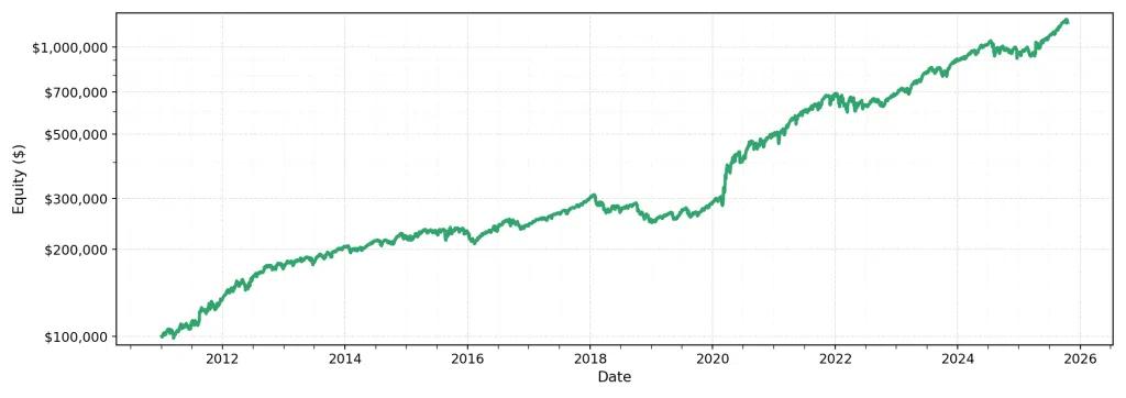
Portfolio Performance Statistics

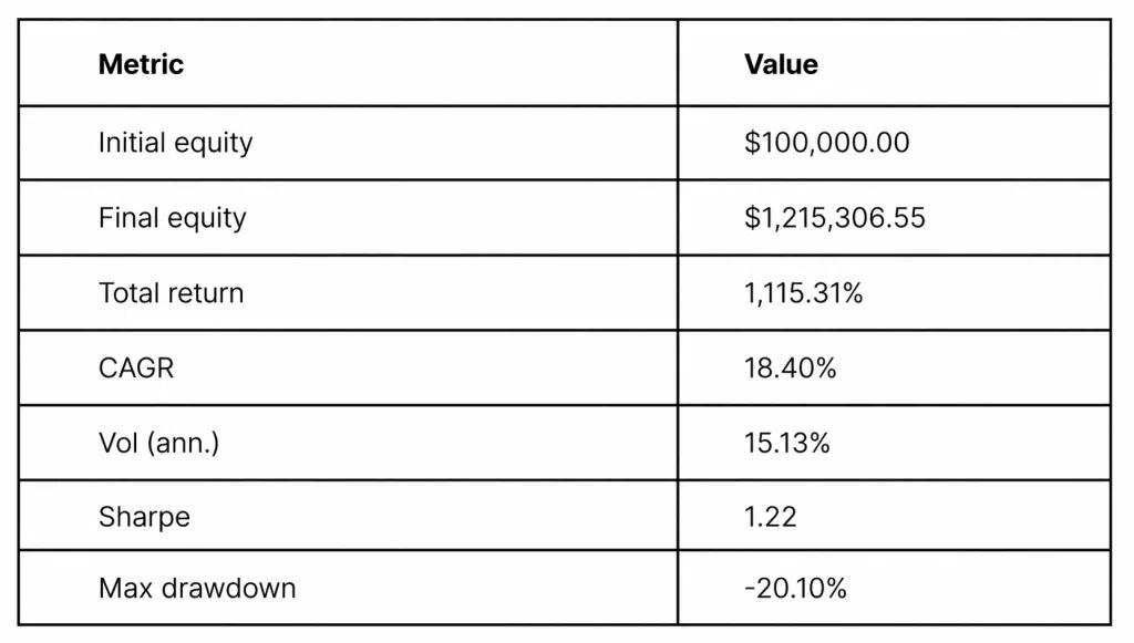
All results shown are based on historical simulations and do not represent actual trading results.

A couple key points about this portfolio:

1. The CAGR of 18.40% is much better than the long term average return of most assets including any of the portfolio components (equities, commodities, volatility risk premium, etc).
2. The portfolio volatility at 15.13% is lower than the market volatility which floats around 16-18%, meaning that the “swings” are a bit smaller on a day to day basis.
3. A max drawdown of 20.11% is about 50% smaller than the max drawdown you would have experienced holding SPX or other equities.
4. A sharpe ratio of 1.22 is an institutional grade return on risk. Typical Sharpes achieved in the market are between 0.5-0.7.

By reading this analysis, it should be clear that this portfolio delivers highly attractive returns, while maintaining lower risk and volatility than other readily available strategies.

Once you combine this with how it only takes a few minutes each week to run, the return on risk and time become extremely attractive.

Portfolio Performance By Year

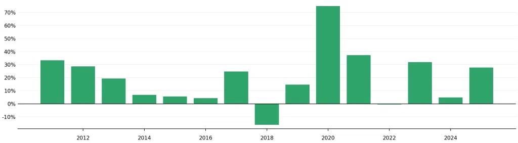
As you can see, most years the strategy sees strong growth. Occasionally we see modest growth. Only once in 15 years did we really end the year in the negative (2018, we were effectively flat in 2022), and only down about 15% compared to many years where the overall market has seen a worse return than that, for example in 2022 when the market ended the year down ~20%.

Performance During COVID and Bear Markets

One other thing that is interesting to note is that the best performing year was actually in 2020. The reason I want to point this out is that it highlights one of the most important functions of this portfolio, which is that built into the VIX strategy is a signal that flips our position from being short volatility (make money when things are calm) to long volatility (make money when things are crazy). Because of this signal, we were able to not only avoid the COVID crash, but actually monetize it greatly.

Note: it is also important to note that we only have one event of “COVID level proportions” to examine in the research since VXX did not exist for 2000, 2008, etc. For this reason, it is also important to understand the reasoning behind the “flip to long” signal, and why it’s reasonable to expect it to be effective in the future. The exact details of how this works are outlined in the VIX Strategy portion of this research.

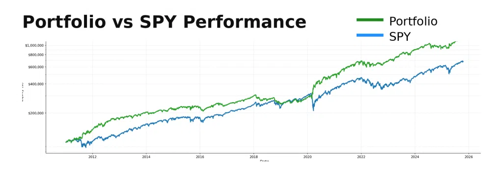
Comparison to SPY - Timeseries

The chart below shows how the portfolio performed relative to SPY. Note that it uses a log scale, which makes it easier to compare performance over a multi-year period. As you can see, the portfolio’s compounding leads to significant outperformance versus traditional buy and hold.

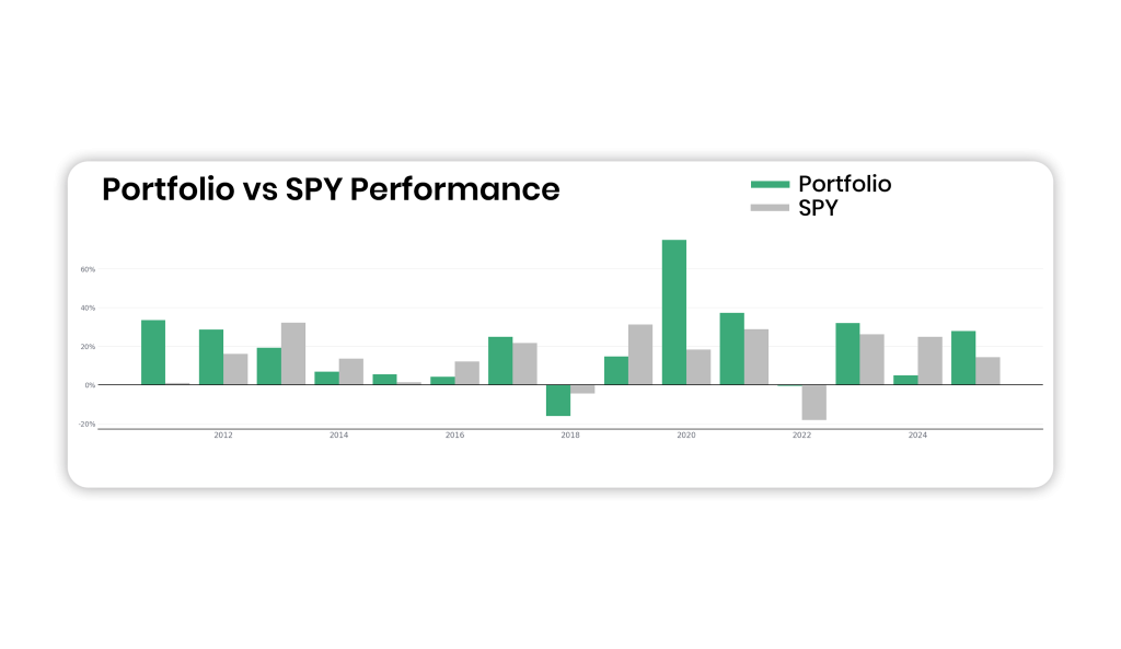
Comparison to SPY - Year by Year

Comparing the fiscal year performance from 2011 – 2025 for the PA portfolio and SPY, we can see that:

• Portfolio outperforms SPY 9/15 of years (60% of the time)
• The strategy was profitable 13/15 years (87% of the time)
• It’s worst year (2018) was better than SPY’s worst year (2022)
• Extreme bear market scenarios are highly profitable (2020) because of how the VIX Strategy works

Something that is really important to note when looking at the performacne of the PA portfolio is that not every year is profitable, and not every year outperforms benchmarks that we may use like SPY.

That said, when you looking at a multi-year period, not only do we see outperformance, we see such a significant level of outperformance that by the end we’ve earned almost double the amount of returns.

As self directed investors, this is one of the hardest parts about strategy analysis to become comfortable with. When we decide on a system to allocate capital towards, we need to be able to take a multi year view. Short term thinking makes portfolio construction and strategy design almost irrelevant, since neither of which would be given the time to play out.

Monte Carlo Simulations

The chart below shows you the results from the Monte Carlo simulation run on the portfolio. This takes all of the data in our backtest and simulates different potential performance charts that would be possible.

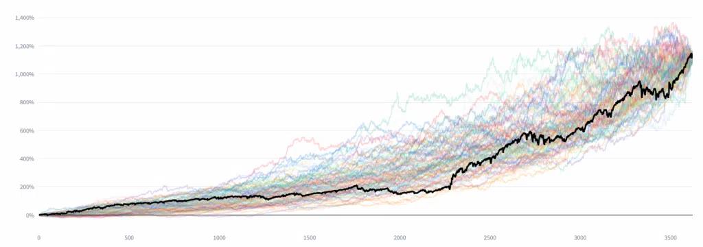
As you can see, performance across all simulations looks excellent, with all variations having a pretty tight range of potential outcomes over time.

How The Portfolio is Traded

General Portfolio Structure and Management

Long 5 ETFs, short 1 ETF. That’s what the portfolio typically looks like. Simple.

There is a weekly rebalancing triggered Fridays at 3:30PM EST.

Occasionally there will be other trades when there is a signal change.

All of this is monitored by the system for you, and total trading time is under 10 minutes per week.

Everything in This Portfolio is Systematic (The Key To Success)

What makes this portfolio truly the first self serve, hedge-fund as a service is that it’s the first portfolio of this caliber that is completely systematic end-to-end.

Every rule is quantified. Trade sizing is quantified.

Even the way you place trades is meticulously selected to be systematic. For every trade, you are placing Market On Close (MOC) orders because Market-On-Close orders execute in the closing auction, all trades are matched at one official final price. This is the same thing that was used in backtesting, which means the trade price assumptions we made in testing will be the same as what you see in practice.

This is one of the things that has always been the major flaw in strategies for retail traders. The results that looked so good in testing were not replicable in practice. A combination of complexity, overly generous assumptions, and practical differences lead to wildly different results as risk profiles.

This is a major obstacle that the complete systemization of this portfolio allows us, and our members, to overcome.

How Your Capital is Allocated to Portfolio Positions

Assume you have $10,000 in a margin account.

That $10,000 is your portfolio value, or NAV. Every position in the portfolio is sized as a percentage of that total value.

The system determines how much exposure to allocate to the ETF sleeve and how much to allocate to the VIX sleeve, all based on that same NAV.

Because this is a margin account, total exposure will usually exceed $10,000. That is by design. However, the amount of margin used is controlled. Most brokers allow up to 200% exposure relative to your capital. This portfolio typically uses far less, and the VIX Strategy (The one that most people have questions about) is capped at 40% of NAV.

In other words, margin is used as a tool, not as aggressive leverage.

When you begin, the system calculates the exact number of shares to buy or sell for each ETF based on your current NAV and active signals.

From there, you are guided through weekly rebalancing and occasional signal changes. In practice, you are simply trading ETF shares according to a structured plan.

ETF Strategy Research

The All Weather Portfolio

The ETF Strategy uses an “All Weather ETF portfolio”, inspired by Ray Dalio’s ideas, and combines it with an “Asset Momentum Signal” inspired by Rob Carver.

Ray Dalio’s All Weather portfolio exists because different assets win in different economic conditions, and no one can reliably predict which regime is coming next. By holding assets that benefit from growth, recession, inflation, and deflation at the same time, the portfolio is designed to survive any environment rather than bet on one.

In our portfolio we hold:

• Equities (SPY)
• Gold (GLD)
• Bonds (TLT)
• Commodities (DBC)
• Currencies (FXE)

The weights for these positions are not equal. They are scaled in proportion to how strong the premium is in the asset class, and are as follows:

• SPY: 35%
• GLD: 20%
• TLT: 30%
• DBC: 5%
• FXE: 10%

Asset Momentum Overlay

Rob Carver’s momentum across asset classes exists because markets tend to move in trends, not in perfectly random jumps. Using rules to hold assets that are rising and reduce exposure to those falling lets the portfolio adapt automatically instead of relying on forecasts.

We apply a long-term trend-following signal based on the relationship between shorter-term and longer-term price averages. The parameters are set to reflect meaningful market time horizons and are intentionally fixed, rather than optimized for backtest performance, to ensure robustness out of sample.

The specific implementation of this signal is proprietary, but the underlying principle remains simple and consistent across all assets:

When the shorter-term trend weakens relative to the longer-term trend for a given asset, the position is reduced to cash. Exposure is only reintroduced once the trend re-establishes itself.

By combining this with The ETF Strategy’s broader portfolio construction, we create a highly stable return profile that serves as the foundation, or “anchor,” of the overall portfolio.

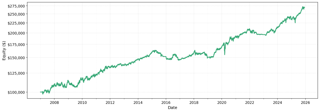
ETF Performance and Role

Here is what the performance for this strategy looks like:

2007 - 2025 ETF Strategy Performance Chart

2007 - 2025 ETF Strategy Key Metrics

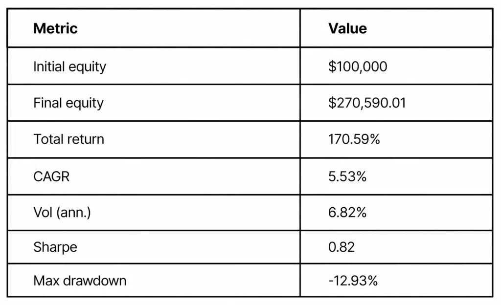
Understanding the return profile: Reliable returns and controlled risk

You may look at this and think that the CAGR is too low. But you must remember, that this strategy is the foundation of the portfolio, not the entire thing. Look at how low its annualized volatility is. A max drawdown of only 12.93%! It’s important to note that for this data set, we see 2008, which is when SPX had a drawdown of ~50%! In contrast, we saw a drawdown that is just a fraction of that.

This is a very stable strategy, and that is what makes it such a good “ingredient” in our portfolio. If you refer back to the top, where we have the portfolio performance, you will be reminded how well the overall portfolio performs, and that this is a pivotal ingredient in creating that return profile.

Note: The reason the ETF strategy data goes back to 2008, while the portfolio backtest and VIX data go back to 2011 is because the data needed for the VIX strategy only started tracking in 2011.

VIX Strategy Research

Our second strategy is based on trading the VIX Futures curve, an approach commonly called the “VIX Term Structure Roll-Down Yield”. This one gets a bit more technical to understand, so just remember that the math behind this is all handled for you.

VIX Performance and Role

Here is what the performance for this strategy looks like:

2011 - 2025 VIX Strategy Performance Chart

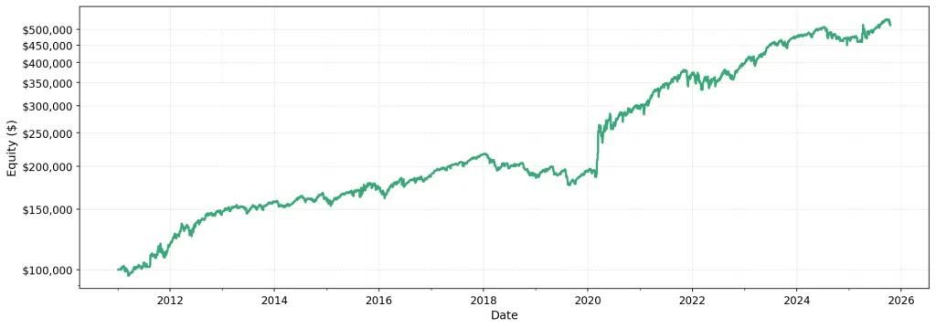
2011 - 2025 VIX Strategy Key Metrics

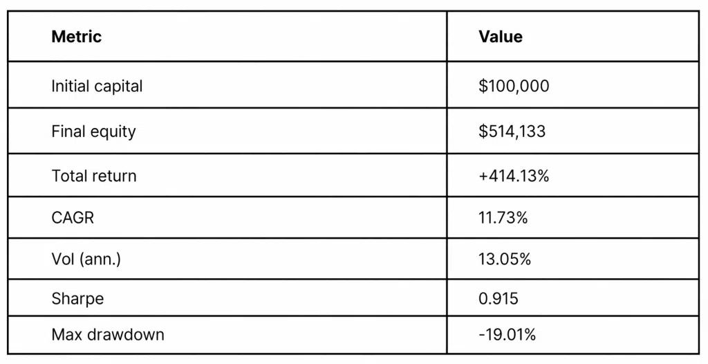
As you can see, the CAGR for this strategy is significantly higher than with the ETF Strategy. And as expected, this comes with a higher Max drawdown and volatility. It’s important to note that the volatility and drawdowns are still lower than market averages. This strategy draws on a different “source of returns” than the ETF Strategy, and combined with the “crash protection” component, it makes it a very attractive compliment to add to our portfolio.

VIX Term Structure and Roll-Down Yield

VIX term structure roll-down yield exists because investors consistently overpay for future volatility as insurance. When volatility stays normal, futures prices naturally drift lower over time, allowing us to earn a premium for taking that risk. In most market environments, the price of the futures is higher than the “spot price” of VIX, and so as time passes, the futures prices decrease down towards the spot price.

This is what the VIX Futures curve looked like on January 8, 2026.

VIX Term Structure Example

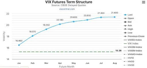
The blue line is the futures prices for each month, and the green line is the current VIX price.

As time passes, the January dot decreases towards the spot price, the February dot decreases towards the January dot (as it becomes the new 1 month), and so on. This is the “rolldown” effect.

And this is what our second strategy is based upon.

To monetize this effect, the position we hold is: Short VXX shares

Signal Framework

The two signals used to decide whether we are short, flat, or long VIX futures exposure are:

1. Volatility Risk Premium (VRP)

This is an estimate of whether things are overpriced or underpriced right now. If implied volatility is higher than what recent price action suggests it should be, traders are likely overpaying for protection, which favors the short VXX position. If it’s lower, shorting volatility is dangerous and so we adjust to cash or long VXX.

2. VIX Term Structure, Contango vs Backwardation

This is a comparison between short-term fear and medium-term fear. If short-term fear is less than medium term fear, we consider it a normal, calm market environment. If short-term fear is greater than medium-term fear, we consider it to be a stressed market, meaning near-term risk is elevated.

Position Decision Logic

Note: all of these calculations are done for you in the platform. We explain it to help you understand what’s going on under the hood.

These two signals are combined to tell us whether conditions are:

1. Favorable for short VXX
2. Favorable for long VXX
3. Indifferent, better to be in cash

Here is how the two signals are combined to determine which position we take:

1. IF VRP is positive AND short-term fear < medium-term fear THEN → Short VXX (high conviction)
2. IF VRP is negative AND short-term fear < medium-term fear THEN → Short VXX (reduced size)
3. IF VRP is negative AND short-term fear > medium-term fear THEN → Long VXX (high conviction)
4. ELSE THEN → Cash (no position)

Based on these rules, here is a graphic showing the % of time that we are typically short, long, or in cash:

% Of Time Long/Short/Flat For VIX Strategy

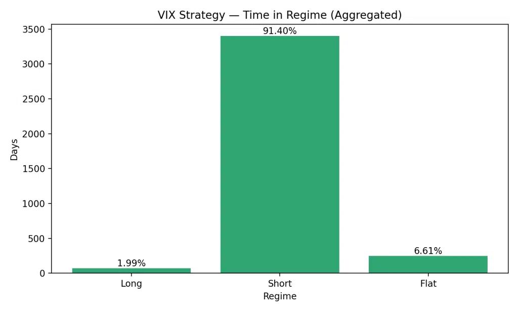
1. The majority of the time (91.40%) we are short VXX, which reflects that most of the time, things are calm.
2. Just 1.99% of the time we are long VXX, which makes sense since it’s quite rare that we are seeing high degrees of market volatility
3. 6.61% of the time we are cash.

Position Sizing Rules

Note: All of these calculations are done for you in the platform. We explain it to help you understand what’s going on under the hood.

Unlike the ETF strategy, which has fixed weighting for each ETF, this one is variable. We adjust the position sizing using the following system:

The strategy risks less when market volatility is low (VIX is low) and more when volatility is already high (VIX is high). This is done because VIX is mean reverting, so as it does, we want more exposure since it can drive greater profits. This is done by using the level of VIX itself as a scaling variable.

The base rule is: the position size scales up as volatility increases, and scales down as volatility decreases.

So if we had $10,000 allocated to the strategy, and VIX was at 15, we would allocate $1,500 to the VXX position, and trade the number of shares that allows.

If VIX jumped to 30, we would increase our position size to $3,000.

If the signal for reduced size is triggered, we reduce the position size by 50% until there is another signal change.

So if we had $10,000 allocated to the strategy, VIX was at 15, and the reduced size signal is active, we would allocate $750 to the VXX position, and trade the number of shares that allows.

Note: Position size for VXX is capped at 40% of NAV. If it exceeds this, it triggers a rebalancing to bring down position size.

Backtest Realism and Assumptions

When analyzing a backtest and strategy design there are two things that you need to consider, in order to understand if the test you are seeing is a realistic representation of the returns you could have achieved.

1. Assumptions
2. Backtest design choices to ensure realistic results
3. Process for arriving at signals and rules

The reason these must be considered is because if the assumptions are too “generous” , then the results are likely inflated and returns could be much lower.

And if the process for arriving at signals / rules is completely arbitrary, then they may be overfit (meaning that they are unlikely to work in practice).

Assumptions In Our Testing

Included below is a list of assumptions made in our testing. Three assumptions we had to make were regarding commissions, slippage and borrow rates. Commissions are the amount that someone pays their brokerage to place a trade. Slippage is the difference between the mid price and the price you get filled at. Borrow rates are the interest you pay in order to short shares (we are short VXX a lot of time)

1. Slippage assumed: $0.00

Reasoning: Trades are placed using Market On Close (MOC) orders.

Because Market-On-Close orders execute in the closing auction, all trades are matched at one official final price. Your backtest uses that same closing price, so there’s no difference between expected and actual fills, meaning slippage isn’t a factor. Since we are trading highly liquid ETFs at a size too small to influence the auction, we won’t move the market anyway.

2. Commissions assumed: $0.005 (half a cent) per share.

Reasoning: Trading ETFs is free at most brokerages, so can assume 0 commissions here. Nevertheless, we assumed half a cent, or $0.005 fee per share traded.

3. Borrow rate assumed: 3.5%

Reasoning: Since we are shorting the VXX ETF, we had to make an assumption about the borrow rate. We looked historically and assumed an average borrow rate of 3.5% to put into our model.

4. Signals generated at 3:30PM EST, Signal Time VS Fill Time

Signals are generated at 3:30pm ET using only data available at that time. Prior-day closing prices may be used, but the current day’s official closing price is not included in signal construction. Trades are then executed using market-on-close orders. This ensures no lookahead bias is present in the backtest.

Backtest Design Choices to Ensure Realistic Results

1. Avoiding forward looking signals

Signals are generated at 3:30PM EST using only data available at that time. To avoid using any data or insight that would not be available at the time of signal generation in reality, we took the following steps:

For signal calculations that require historical analysis, we use prior-day closing prices, but the current day’s official closing price was not used in signal construction. For the price data of the “signal day” needed, we used the 3:30PM EST time stamp’s data.

2. Signal generation & trade execution occur at different times

Signals are generated at 3:30PM EST, while trades are executed at 4:00PM EST. This avoids the unrealistic assumption that a trader can observe market data, generate a signal, place an order, and receive a fill at the exact same instant. The sequence in the backtest matches the sequence in real trading: decide first, execute second.

3. Test: Backtest margin of error using MOC fills , 3:30PM sizing is acceptable

One question when looking to implement this portfolio live is if there is a statistically significant different between determining number of shares traded at 3:30PM EST or 4:00PM EST. The reason this is important is because we have fixed or “pre determined” weights for each of the ETFs, the signal comes at 3:30PM EST, but then trades are not actually executed until 4:00PM EST.

Position sizing should in practice be determined at 3:30PM EST, but then there is the possibility of price drift in the final 30 minutes of the day, which could result in divergence from the theoretical returns. This is why testing is required.

The image below shows the results of our test in which we analyzed the difference between calculating the number of shares to be traded during signal changes and rebalances at 3:30PM EST vs 4:00PM EST.

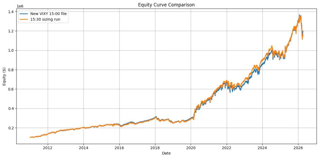
Blue line: signal 3:30PM EST, size at 3:30PM EST, fill at 4:00PM EST

Orange line: signal 3:30PM EST, size 4:00PM EST, fill 4:00PM EST

As you can see, there is no clear divergence that occurs between the two lines. During ~2022, you can see 1-2 days where a divergence occurs, and then it stays that way. Then in 2025, the same thing happens but this time the opposite line performs better, then stays this way. This indicates that what we are seeing is just variance and that sizing trades at 3:30PM EST and executing them at 4:00PM EST does not impact the strategy in a meaningful way.

4. Avoiding over optimization of signals

If a rule like a moving average crossover truly adds value, it should work broadly, not just at one exact parameter setting.

This principle was applied across all strategy rules, not just moving averages. Parameters were chosen based on clear, defensible reasoning, and were not tuned to maximize historical performance.

The goal is not to produce the best-looking backtest, but to ensure the strategy captures real, persistent effects that are more likely to hold up out of sample.

Critiquing Our Process - Understanding Signal Design

There were two steps that we took when determining the rules for each strategy.

1. Start With Logic

Before even looking at the data, we asked ourselves: does this rule make sense? For example, it makes sense when recent performance is worse than the long term average, things tend to underperform. It’s a reasonable thought. Likewise, it’s reasonable to think that when the VIX term structure is in contango (normal, downward sloping) that the volatility risk premium should be there. Each of the rules in our system start with a similar notion, and beyond that, typically are evidenced in the professional trading space by being implemented in hedge fund strategies.

2. Test The Robustness of The Data

Now it’s time to ‘quantify’ each of the rules, and then add them to the model to see if they improve returns. What people trying to make a ‘pretty’ backtest will often do is try many variations of the signal and then present the one that achieved the best performance. For example, they use a moving average crossover, and then change the moving averages by one day many times, to see which one outputs the highest return. But this would be an example of what we call overfitting, or put simply, manipulating the data to make it look better than it is.

We have to remember, that mixed in with the signals is still a lot of noise, a lot of randomness. So when we make these “micro changes” and try to optimize, yes, it is likely we will find one that does better than the others by a bit, but it’s almost certainly randomness. Because it doesn’t make sense why changing the moving average by one day (and doing this hundreds of times) and then picking the one that did the best should actually improve your returns. We are forgetting to start with “logic first”.

So instead, we do the opposite. We also test multiple variations of what the signal could be, but instead of just picking the best one, what we are doing is making sure that regardless of which variation we pick, the edge persists. This is actually a test we run to confirm that our original logic is correct. Because if it is, these “micro changes” should not destroy the edge.

Conclusion

This portfolio is built to do three things. Deliver strong returns with lower risk than the market, keep you confident enough to keep adding capital, and make compounding realistic over the years.

It’s an all-weather ETF base, plus a volatility strategy that monetizes calm markets and flips defensive when markets get stressed.

It delivers a growth rate of 18.40%, with a max drawdown of just 20.10%. It has lower volatility than the market, and a Sharpe ratio of 1.22.

It turned COVID into the most profitable period it has seen, and even turned the -20% bear market in 2022 into a flat year. The fact that it provides some crash insurance is good, and that it turns it into a profit rather than just softening the blow is great.

Beyond the performance metrics, what’s most important to note is that there is no “magic” in this strategy. It’s built on logical ideas that are seen and used in the professional space. It’s rules based so there’s no guessing, or gut feelings. The execution is simple (you are just trading ETF shares) and it survives (sometimes even thrives) in bad market environments.

All that said, the strategy is not “free money”, and one should still expect drawdowns, and periods of slow performance. Most years will be quite boring, and that’s actually part of the point. This is not about the dream of the home run. It’s about doing something that actually works, and can deliver results that make the time invested truly worthwhile.

If you are looking for excitement, this isn’t it. But if you want a portfolio you can run for years and actually stick with, this is a realistic way to do it. The setup and management is straightforward. And once in place, it is something you can feel confident contributing capital to over time, knowing it is grounded in sound logic and durable ideas.